In this module, we'll introduce you to the core statistics you'll be using in your analysis and an approach for your analysis.
Home | Lesson 1 | Lesson 2 | Lesson 3 | Lesson 4 | Lesson 5
Raw & Calculated Hockey Stats
The EP Draft Center has limited raw hockey statistics on minor-league players. For example, their standard view includes Games Played (GP), Goals (G), Assists (A), Points (TP), and Penalties in Minutes (PIM).
However, with just this limited set of raw statistics, you can calculate some 'per-game' statistics; that is, Goals per Game, Assists per Game, Points per Game, and PIM per Game. You can also apply the NHLe score to Points per Game and get a standardized way of looking at productivity.
At this point, it's helpful to return to the big question for a second because the answer to a sports question should have context associated with it. If you've forgotten, it is:
Who are the top 10 forward incoming NHL 2026 Draft prospects, ranked by Points per Game?
For example, your analysis might produce the top 10 forwards ranked by Points per Game, but by including Goals per Game, Assists per Game and PIM per Game, you begin to get a second-level perspective on a player's strengths and weaknesses. You begin to see where a player could be a playmaker or goal-scorer – thus align players strategically to other player's strengths or weaknesses.
Take Marcus Nordmark, for example, who is performing above the average Adjusted PPG (ADJ PPG) in the top quartile of our dataset (which is 0.380). He can convert, but is over twice as strong in his passing game. So, overall he has a strong Adjusted PPG of 0.382. However, he also has the highest PIM per Game (PIMPG) in the top 100. He's a decent size at 6'2" and 187 pounds, but is the high number of penalties a problem or would it self-correct in the NHL?
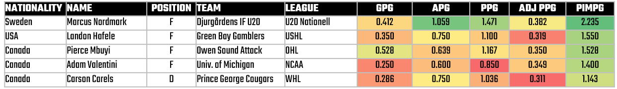
This is the value of a simple summary heatmap; you can see where and how players' games and styles differ. Note that all of this, regardless of whether a player is strong or weak, warrants additional research and exploration.
So, we come back to the idea again that Points per Game (in this case Adjusted Points per Game) are not treated equally – and require secondary analysis to ensure you have the context.
So, What's Our Approach Then?
With a sense of the stats available to you in the dataset, the question now is what is our approach (and methodology). Here again we return to the question we're trying to answer to better arm ourselves with the right methodology.
That said, our general approach will be as follows:
- Create a heatmap view to identify high-level areas of strengths and weaknesses (around production).
- Divide the forward cohort into quartiles and compare.
- Explore the distribution of the Adjusted Points per Game for a statistical level set.
- Use player z-scores to discover any outliers.
- Implement a K-means cluster analysis to find the 'elite' clusters.
You may want a different approach, but the above gives us:
- A way to move from high-level to a more detailed level;
- Categorized groupings across the dataset (so we can build a comparative view); and
- Both a simple and algorithmically-driven way to cluster the cohort to triangulate our findings.
Thus, our approach represents the 5 steps above and our methodology is to use the Adjusted Points per Game as a key calculated (and standardized) statistic for a univariate ranking categorization and more advanced grouping using z-scores and a clustering algorithm.
You could choose to stick only with Excel and focus on the first 3 steps, and you'd likely be fine. However, we've found that additional analyses can uncover interesting finds and confirm your initial analysis. However, you would likely need some programming skills in R (or Python) to implement the final two steps.
What Now?
So far, we've covered the big question we're trying to answer, curating the dataset, and the stats and methodology. We're now ready to move onto the data analysis phase. This is where we'll implement the approach and methodology from this lesson.
Okay, let's get started!
👉 Up Next? Lesson 4: Data Analysis & Visualizations